(530h) Using Deep Learning to Predict the Permeability of Porous Media

Introduction

Understanding of the properties of porous media is beneficial to a range of applications including fuel cells [1] and automotive exhaust treatment [2]. Determining porous media properties, such as permeability or effective diffusivity, typically require some type of pore-scale fluid simulation. Common approaches include finite volume Computational Fluid Dynamics (CFD) [2] or the Lattice Boltzmann Method (LBM) [3]. Both methods have their benefits, but they can be computationally expensive and often require High Performance Computing (HPC) clusters, especially when considering porous media that are of Representative Elementary Volume (REV) scale. Therefore, the use of deep learning to predict porous media properties has become a popular area of research.

By far the most common architecture choice for porous media property prediction is the Convolutional Neural Network (CNN) [4–6]. Porous media are often represented as images, in either 2D or 3D, which makes the CNN an ideal choice for porous media deep learning models. However, they can become computationally expensive when using 3D convolutional layers for 3D porous media, which is a problem because properties of 3D porous media are not necessarily represented by their 2D projections. An alternative approach to the CNN is the Graph Neural Network (GNN) [7]. The GNN architecture allows for graph data to be input into a neural network which then predicts some desired property. This is well suited to porous media research because the pore networks extracted from porous media images can be represented as graphs.

Regardless of the architecture choice, training a deep learning model on porous media samples that are of the REV-scale requires large and complex models. This work describes the process for training a GNN to predict the permeability of both industrially relevant manufactured materials and rock samples using multiple GPUs on a HPC cluster. The inference time of the model was then compared with the LBM.

Methods

Deep learning models for porous media property prediction typically require thousands of training samples. This is due to the inherent complexity of the input data for the models – representative porous media samples can quickly become large. Obtaining a dataset of real porous media samples is expensive due to the imaging requirements, with methods such as X-ray tomography often taking hours per sample [2]. Similarly, obtaining the ground truth for the property of interest is often time consuming with both experimental techniques and pore-scale simulations. This presents difficulties for preparing a suitably large and varied dataset, which is essential for an accurate and generalisable model.

Dataset Preparation

A set of porous media samples was obtained, comprising both real and non-real porous media. Following this, a REV-scale study was performed to determine whether the samples were large enough, then a sampling data augmentation approach was used to extract a dataset of smaller, representative sub-samples from the set of parent structures. This allowed a large and varied dataset of both real and non-real porous media to be generated. The LBM was used to simulate flow through each sample to determine the permeability, the target property for the GNN, which was validated against experimental permeability data.

As with any machine learning model, data leakage can cause a model to appear to have high accuracy but can often lead to a model that is unable to generalise to new, unseen structures. To remove the risk of data leakage in the model, three independent sets of parent structures were generated: one for training, one for validation during hyperparameter tuning and one completely unseen set for testing purposes. Sub-samples were extracted from each unique parent structure after partition, removing the risk of data leakage during data augmentation.

Graph Neural Network

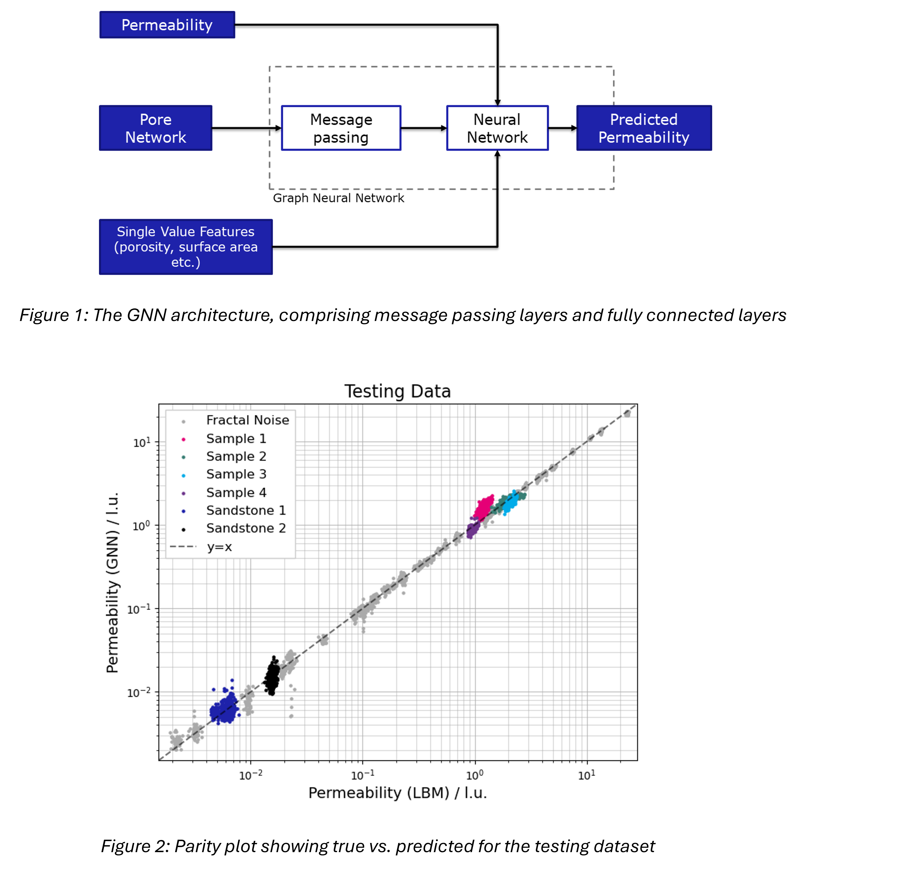
A GNN was developed using PyTorch Geometric [8] and PyTorch [9] which allowed for large and complex models to be trained using distributed training with multiple GPUs. The GNN required the pore network to be encoded into a feature matrix, comprising pore features and an adjacency matrix, which encodes the connectivity of the pore network. The adjacency matrix was weighted with the length of the pore connections. The GNN is split into two main sections: a set of message-passing layers and a set of fully connected layers. Figure 1 shows how the two layers and input features are connected. The purpose of the message passing layers are to encode node features and the adjacency matrix into a set of updated node features and the fully connected layers relate the updated features to the permeability. An optimal set of hyperparameters was selected using Optuna [10], using the Mean Squared Error (MSE) on the validation dataset to optimise the model. Finally, a model was trained using the optimal hyperparameters and tested on the unseen testing dataset.

Results

Three independent datasets, each comprising a mix of non-real fractal noise structures, some sandstone samples from the Digital Rock Portal [11] and some anonymised porous media samples were generated. The permeability of each parent structure was obtained using a C++ LBM library, Palabos [12]. The sub-sampling data augmentation approach yielded between 500-1000 representative samples from each of the porous structures in the datasets. In total, there were 115,000 training samples, 33,000 validation samples and 31,000 testing samples. Most of the samples in each dataset were fractal noise, with around 10-20% in each dataset being real samples.

Once the optimal set of hyperparameters had been found, a new model was trained and tested on the third, unseen testing dataset. The GNN showed a good agreement with the permeability calculated from the LBM simulations, which was trained to predict the natural logarithm of the permeability. This was to ensure the high permeability samples were weighted equally with low permeability samples. The GNN had an MSE of 0.0179, which is significantly better than the Carman-Kozeny equation [13] with a MSE of 6.45. Figure 2 shows the parity plot for the LBM permeability (true) and the GNN permeability (predicted) in lattice units. The LBM is inherently dimensionless with the use of conversion factors to switch between physical units and lattice units. Physical length scale has been omitted from this work to anonymise the samples. Given the model is trained to predict the lattice unit values without the need for conversion factors, it allows the model to be independent of the resolution of the input porous media samples. If the voxel size of a sample is known, the lattice unit permeability can be converted to physical units. The GNN was also able to make permeability predictions in near real-time, providing the pore network is available, whereas the LBM simulations typically required hours of simulation time to complete. Even with pore network extraction times included, the LBM was over 10 times slower.

Conclusions

In this work, a GNN was trained to predict the permeability of both non-real and real, representative porous media samples. This method allows for rapid prediction of the permeability based on the pore networks extracted from the samples. The GNN was able to significantly out-perform the commonly used Carmen-Kozeny equation when comparing to the LBM ground truth, while making the predictions significantly faster than the LBM.

References

[1] Z. Niu, V. J. Pinfield, B. Wu, H. Wang, K. Jiao, D. Y. C. Leung, and J. Xuan, Energy Environ. Sci. 14, 2549 (2021).

[2] P. Kočí, M. Isoz, M. Plachá, A. Arvajová, M. Václavík, M. Svoboda, E. Price, V. Novák, and D. Thompsett, Catal. Today 320, 165 (2019).

[3] A. Eshghinejadfard, L. Daróczy, G. Janiga, and D. Thévenin, Int. J. Heat Fluid Flow 62, 93 (2016).

[4] H. Wang, Y. Yin, X. Y. Hui, J. Q. Bai, and Z. G. Qu, Energy AI 2, 100035 (2020).

[5] H. Wu, W.-Z. Fang, Q. Kang, W.-Q. Tao, and R. Qiao, Sci. Rep. 9, 20387 (2019).

[6] A. Rabbani, M. Babaei, R. Shams, Y. D. Wang, and T. Chung, Adv. Water Resour. 146, 103787 (2020).

[7] C. Cai, N. Vlassis, L. Magee, R. Ma, Z. Xiong, B. Bahmani, T.-F. Wong, Y. Wang, and W. Sun, Int. J. Multiscale Comput. Eng. (2021).

[8] M. Fey and J. E. Lenssen, in ICLR Workshop on Representation Learning on Graphs and Manifolds (2019).

[9] A. Paszke, S. Gross, F. Massa, A. Lerer, J. Bradbury, G. Chanan, T. Killeen, Z. Lin, N. Gimelshein, L. Antiga, A. Desmaison, A. Köpf, E. Yang, Z. DeVito, M. Raison, A. Tejani, S. Chilamkurthy, B. Steiner, L. Fang, J. Bai, and S. Chintala, ArXiv191201703 Cs Stat (2019).

[10] T. Akiba, S. Sano, T. Yanase, T. Ohta, and M. Koyama, .

[11] M. Prodanovic, M. Esteva, M. Hanlon, G. Nanda, and P. Agarwal, (2015).

[12] J. Latt, O. Malaspinas, D. Kontaxakis, A. Parmigiani, D. Lagrava, F. Brogi, M. B. Belgacem, Y. Thorimbert, S. Leclaire, S. Li, F. Marson, J. Lemus, C. Kotsalos, R. Conradin, C. Coreixas, R. Petkantchin, F. Raynaud, J. Beny, and B. Chopard, Comput. Math. Appl. 81, 334 (2021).

[13] P. C. Carman, Chem. Eng. Res. Des. 75, S32 (1997).