2025 AIChE Annual Meeting
(452b) Pinn-Based Simulation of Ceramic Firing Process Under Various Thermal Profiles
To optimally design and control manufacturing processes, precise first-principles models are essential. Many processes are modeled by partial differential equations (PDEs), which are solved with numerical techniques such as the finite element method (FEM). Although FEM simulations accurately capture spatial and temporal dynamics, they require substantial computational resources. Consequently, there is growing interest in surrogate models that retain the physical fidelity of first‑principles models while dramatically reducing the computational cost.
Raissi et al. [1] proposed Physics-Informed Neural Networks (PINNs), which are deep learning models that incorporate physical constraints into their training objectives. PINNs can solve forward problems governed by PDEs, similar to numerical solvers, without reliance on large datasets. Additionally, PINNs can flexibly integrate experimental data to accelerate model training. Wurth et al. [2] showed that applying a PINN model to composite material manufacturing process optimization can reduce computation time by several hundred times compared to traditional FEMs when repeatedly evaluating different settings.
In this research, we focus on the firing process of ceramics manufacturing. Ceramics manufacturing involves shaping and thermally treating materials such as clay, alumina, and other inorganic compounds to produce products ranging from construction materials to high-performance components used in electronics and energy devices. Among its various stages, the firing process is energy-intensive and accounts for over 60% of the total CO2 emissions in ceramics production. Although this stage requires temperatures above 1000℃ to achieve the desired material properties, it typically employs a slow heating process to prevent defects caused by steep internal temperature gradients. The current heating rate is conservatively designed to ensure product quality; thus, optimizing the temperature rise profile is expected to reduce CO2 emissions.
We adopt a two-step framework to optimize the operating conditions of the firing process. The first step is to estimate temperature distributions inside the product because they cannot be measured. The second step is to optimize heating rates that satisfy temperature uniformity constraints inside the product. This study focuses on the first step and aims to develop a high-performance temperature prediction model by employing PINNs. We assess the prediction accuracy of the model by comparing it with the FEM.
Methods
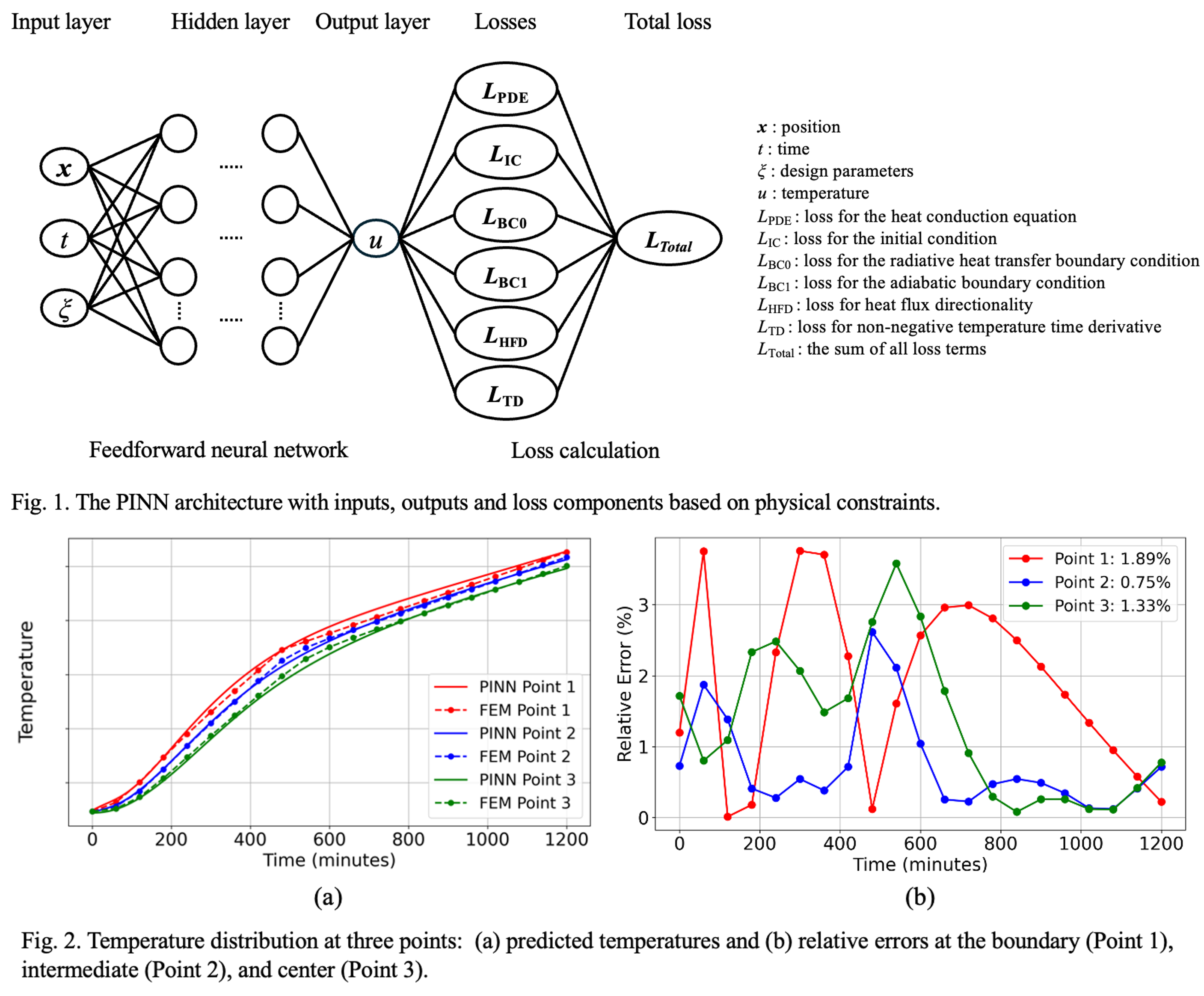
The PINN architecture used in our research is shown in Fig. 1: a feedforward neural network that takes as input the position x, time t, and parameters ξ, which include heating rates and the transition point, and outputs the temperature u. The loss function includes multiple terms that penalize deviations from physical constraints: initial conditions LIC, radiative heat transfer boundary conditions LBC0, adiabatic boundary conditions LBC1, the governing PDE LPDE, heat flux directionality LHFD, and the temperature time derivative LTD. Each term is formulated as the sum of mean squared errors. LIC enforces that the predicted temperature at t = 0 matches the actual initial temperature throughout the domain. For LBC0, heat flux conditions based on the Stefan-Boltzmann law are implemented, where the conductive heat flux at the boundary equals the radiative heat flux from the furnace. The resulting nonlinear equations are solved using a relaxation-based iterative method. LBC1 enforces that the temperature gradient normal to the boundary surface becomes zero. LPDE enforces that the predicted temperature field satisfies the heat conduction equation as the governing equation throughout the interior domain. LHFD ensures that heat flows from high-temperature to low-temperature regions, specifically from the outside to the inside of the product in our target process. LTD ensures a monotonically increasing temperature over time, which reflects the continuous heating nature of the process.
We set the learning rate to 1.0e-6 and used Adam as the optimizer and the hyperbolic tangent function as the activation function. In addition, dimensionless scaling was applied to all inputs and physical properties to accelerate convergence and enhance stability during model training. To enhance training efficiency, we implemented a dynamic weighting method to automatically adjust the importance of each loss term according to the training progress. Specifically, the initial and boundary conditions losses were emphasized in the early stages, while the PDE loss became more dominant in the later stages.
Experiments
The target domain was a cylindrical geometry with a circular cross-section in the x-y plane and height along the z-direction. For material properties, temperature-dependent anisotropic thermal conductivity was considered. Thermal conductivity in the z-direction was higher than that in the x- and y-directions, and thermal conductivity in all directions decreased with increasing temperature. Similarly, the temperature dependence of specific heat capacity was also incorporated. A heat flux boundary condition accounting for radiative heat transfer was imposed at the bottom and side surfaces. In contrast, an adiabatic condition was applied at the top surface. During model training, the loss function was evaluated by using 7,480 points for the initial condition, 42,000 points for the radiative heat transfer boundary condition, 20,000 points for the adiabatic boundary condition, and 100,000 points for PDE, heat flux directionality, and temperature time derivative constraints. These points were resampled at each epoch to enforce the physical constraints efficiently. The prediction accuracy of the model was evaluated by comparing the predicted temperature field with numerical calculation results from the FEM.
Results and Discussion
Fig. 2 shows an example of simulation results, in which the temperature profile was modeled as a two-stage heating process starting from room temperature. We compared the model predictions with the FEM simulations at the boundary point, the intermediate point, and the center point. Fig. 2(a) presents the temperature evolution over time, while Fig. 2(b) displays the relative errors. The mean relative errors at the three points were 1.89%, 0.75%, and 1.33%, respectively. Model training successfully converged with all loss components reaching low values. These results confirmed that the proposed model provides accurate temperature predictions throughout the entire domain.
Despite the promising results, there remains room for improvement. First, regarding the network architecture, Li et al. [3] mentioned that using residual neural networks increases both the training stability and the convergence speed. Also, Xu et al. [4] demonstrated that incorporating convolutional layers into the PINN architecture is beneficial. These improvements are worth considering in future work. Second, the iterative method used to solve the radiative heat transfer boundary condition could be improved by introducing more stable and faster-converging algebraic solvers. Third, the modeling framework should be extended to more complex modeling scenarios. While this study focused on the temperature distribution dynamics of a single ceramic product, actual manufacturing processes involve multiple ceramic products arranged within a high-temperature furnace. A more comprehensive model should account for both the products and the furnace environment to represent the thermal interactions in industrial settings more accurately.
Conclusion
This study developed a temperature distribution prediction model for cylindrical ceramic products during a two-stage heating process using PINNs. We compared our model with the FEM simulations and found mean relative errors below 2% across different locations. Our future work will focus on improving the prediction performance, extending the approach to more complex industrial scenarios, and optimizing heating rates by utilizing our PINN model.
Acknowledgment
This article is based on results obtained from a project, JPNP14004, subsidized by the New Energy and Industrial Technology Development Organization (NEDO).
References
[1] M. Raissi et al., “Physics-informed neural network: A deep learning framework for solving forward and inverse problems involving nonlinear partial differential equations,” J. Comput. Phys., vol. 378, pp. 686-707, 2019.
[2] T. Wurth et al., “Physics-informed neural networks for data-free surrogate modelling and engineering optimization – An example from composite manufacturing,” Mater. Des., vol. 231, p. 112034, 2023.
[3] S. Li et al., “A physics-informed neural network framework to predict 3D temperature field without labeled data in process of laser metal deposition,” Eng. Appl. Artif. Intell., vol. 120, p. 105908, 2023.
[4] J. Xu et al., “Physics-informed neural networks for studying heat transfer in porous media,” Int. J. Heat Mass Transf., vol. 217, p. 124671, 2023.